Complex polytope

In geometry, a complex polytope is a generalization of a polytope in real space to an analogous structure in a complex Hilbert space, where each real dimension is accompanied by an imaginary one.

A complex polytope may be understood as a collection of complex points, lines, planes, and so on, where every point is the junction of multiple lines, every line of multiple planes, and so on.

Precise definitions exist only for the regular complex polytopes, which are configurations. The regular complex polytopes have been completely characterized, and can be described using a symbolic notation developed by Coxeter.

Some complex polytopes which are not fully regular have also been described.

Definitions and introduction

The complex line ${\displaystyle \mathbb {C} ^{1}}$ has one dimension with real coordinates and another with imaginary coordinates. Applying real coordinates to both dimensions is said to give it two dimensions over the real numbers. A real plane, with the imaginary axis labelled as such, is called an Argand diagram. Because of this it is sometimes called the complex plane. Complex 2-space (also sometimes called the complex plane) is thus a four-dimensional space over the reals, and so on in higher dimensions.

A complex n-polytope in complex n-space is the analogue of a real n-polytope in real n-space.

There is no natural complex analogue of the ordering of points on a real line (or of the associated combinatorial properties). Because of this a complex polytope cannot be seen as a contiguous surface and it does not bound an interior in the way that a real polytope does.

In the case of regular polytopes, a precise definition can be made by using the notion of symmetry. For any regular polytope the symmetry group (here a complex reflection group, called a Shephard group) acts transitively on the flags, that is, on the nested sequences of a point contained in a line contained in a plane and so on.

More fully, say that a collection P of affine subspaces (or flats) of a complex unitary space V of dimension n is a regular complex polytope if it meets the following conditions:^[1][2]

• for every −1 ≤ i < j < k ≤ n, if F is a flat in P of dimension i and H is a flat in P of dimension k such that F ⊂ H then there are at least two flats G in P of dimension j such that F ⊂ G ⊂ H;
• for every i, j such that −1 ≤ i < j − 2, j ≤ n, if F ⊂ G are flats of P of dimensions i, j, then the set of flats between F and G is connected, in the sense that one can get from any member of this set to any other by a sequence of containments; and
• the subset of unitary transformations of V that fix P are transitive on the flags F₀ ⊂ F₁ ⊂ … ⊂F_n of flats of P (with F_i of dimension i for all i).

(Here, a flat of dimension −1 is taken to mean the empty set.) Thus, by definition, regular complex polytopes are configurations in complex unitary space.

The regular complex polytopes were discovered by Shephard (1952), and the theory was further developed by Coxeter (1974).

Three views of regular complex polygon ₄{4}₂,

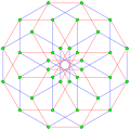
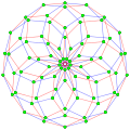
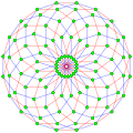
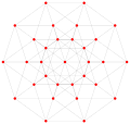
This complex polygon has 8 edges (complex lines), labeled as a..h, and 16 vertices. Four vertices lie in each edge and two edges intersect at each vertex. In the left image, the outlined squares are not elements of the polytope but are included merely to help identify vertices lying in the same complex line. The octagonal perimeter of the left image is not an element of the polytope, but it is a petrie polygon.[3] In the middle image, each edge is represented as a real line and the four vertices in each line can be more clearly seen.

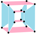
A perspective sketch representing the 16 vertex points as large black dots and the 8 4-edges as bounded squares within each edge. The green path represents the octagonal perimeter of the left hand image.

A complex polytope exists in the complex space of equivalent dimension. For example, the vertices of a complex polygon are points in the complex plane ${\displaystyle \mathbb {C} ^{2}}$, and the edges are complex lines ${\displaystyle \mathbb {C} ^{1}}$ existing as (affine) subspaces of the plane and intersecting at the vertices. Thus, an edge can be given a coordinate system consisting of a single complex number.^{[clarification needed]}

In a regular complex polytope the vertices incident on the edge are arranged symmetrically about their centroid, which is often used as the origin of the edge's coordinate system (in the real case the centroid is just the midpoint of the edge). The symmetry arises from a complex reflection about the centroid; this reflection will leave the magnitude of any vertex unchanged, but change its argument by a fixed amount, moving it to the coordinates of the next vertex in order. So we may assume (after a suitable choice of scale) that the vertices on the edge satisfy the equation ${\displaystyle x^{p}-1=0}$ where p is the number of incident vertices. Thus, in the Argand diagram of the edge, the vertex points lie at the vertices of a regular polygon centered on the origin.

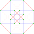
Three real projections of regular complex polygon 4{4}2 are illustrated above, with edges a, b, c, d, e, f, g, h. It has 16 vertices, which for clarity have not been individually marked. Each edge has four vertices and each vertex lies on two edges, hence each edge meets four other edges. In the first diagram, each edge is represented by a square. The sides of the square are not parts of the polygon but are drawn purely to help visually relate the four vertices. The edges are laid out symmetrically. (Note that the diagram looks similar to the B₄ Coxeter plane projection of the tesseract, but it is structurally different).

The middle diagram abandons octagonal symmetry in favour of clarity. Each edge is shown as a real line, and each meeting point of two lines is a vertex. The connectivity between the various edges is clear to see.

The last diagram gives a flavour of the structure projected into three dimensions: the two cubes of vertices are in fact the same size but are seen in perspective at different distances away in the fourth dimension.

Regular complex one-dimensional polytopes

A real 1-dimensional polytope exists as a closed segment in the real line ${\displaystyle \mathbb {R} ^{1}}$, defined by its two end points or vertices in the line. Its Schläfli symbol is {} .

Analogously, a complex 1-polytope exists as a set of p vertex points in the complex line ${\displaystyle \mathbb {C} ^{1}}$. These may be represented as a set of points in an Argand diagram (x,y)=x+iy. A regular complex 1-dimensional polytope _p{} has p (p ≥ 2) vertex points arranged to form a convex regular polygon {p} in the Argand plane.^[4]

Unlike points on the real line, points on the complex line have no natural ordering. Thus, unlike real polytopes, no interior can be defined.^[5] Despite this, complex 1-polytopes are often drawn, as here, as a bounded regular polygon in the Argand plane.

A regular real 1-dimensional polytope is represented by an empty Schläfli symbol {}, or Coxeter-Dynkin diagram . The dot or node of the Coxeter-Dynkin diagram itself represents a reflection generator while the circle around the node means the generator point is not on the reflection, so its reflective image is a distinct point from itself. By extension, a regular complex 1-dimensional polytope in ${\displaystyle \mathbb {C} ^{1}}$ has Coxeter-Dynkin diagram , for any positive integer p, 2 or greater, containing p vertices. p can be suppressed if it is 2. It can also be represented by an empty Schläfli symbol _p{}, }_p{, {}_p, or _p{2}₁. The 1 is a notational placeholder, representing a nonexistent reflection, or a period 1 identity generator. (A 0-polytope, real or complex is a point, and is represented as } {, or ₁{2}₁.)

The symmetry is denoted by the Coxeter diagram , and can alternatively be described in Coxeter notation as _p[], []_p or ]_p[, _p[2]₁ or _p[1]_p. The symmetry is isomorphic to the cyclic group, order p.^[6] The subgroups of _p[] are any whole divisor d, _d[], where d≥2.

A unitary operator generator for is seen as a rotation by 2π/p radians counter clockwise, and a edge is created by sequential applications of a single unitary reflection. A unitary reflection generator for a 1-polytope with p vertices is e^2πi/p = cos(2π/p) + i sin(2π/p). When p = 2, the generator is e^πi = –1, the same as a point reflection in the real plane.

In higher complex polytopes, 1-polytopes form p-edges. A 2-edge is similar to an ordinary real edge, in that it contains two vertices, but need not exist on a real line.

Regular complex polygons

While 1-polytopes can have unlimited p, finite regular complex polygons, excluding the double prism polygons _p{4}₂, are limited to 5-edge (pentagonal edges) elements, and infinite regular apeirogons also include 6-edge (hexagonal edges) elements.

Notations

Shephard's modified Schläfli notation

Shephard originally devised a modified form of Schläfli's notation for regular polytopes. For a polygon bounded by p₁-edges, with a p₂-set as vertex figure and overall symmetry group of order g, we denote the polygon as p₁(g)p₂.

The number of vertices V is then g/p₂ and the number of edges E is g/p₁.

The complex polygon illustrated above has eight square edges (p₁=4) and sixteen vertices (p₂=2). From this we can work out that g = 32, giving the modified Schläfli symbol 4(32)2.

Coxeter's revised modified Schläfli notation

A more modern notation _p1{q}_p2 is due to Coxeter,^[7] and is based on group theory. As a symmetry group, its symbol is _p1[q]_p2.

The symmetry group _p1[q]_p2 is represented by 2 generators R₁, R₂, where: R₁^p₁ = R₂^p₂ = I. If q is even, (R₂R₁)^q/2 = (R₁R₂)^q/2. If q is odd, (R₂R₁)^(q−1)/2R₂ = (R₁R₂)^(q−1)/2R₁. When q is odd, p₁=p₂.

For ₄[4]₂ has R₁⁴ = R₂² = I, (R₂R₁)² = (R₁R₂)².

For ₃[5]₃ has R₁³ = R₂³ = I, (R₂R₁)²R₂ = (R₁R₂)²R₁.

Coxeter-Dynkin diagrams

Coxeter also generalised the use of Coxeter-Dynkin diagrams to complex polytopes, for example the complex polygon _p{q}_r is represented by and the equivalent symmetry group, _p[q]_r, is a ringless diagram . The nodes p and r represent mirrors producing p and r images in the plane. Unlabeled nodes in a diagram have implicit 2 labels. For example, a real regular polygon is ₂{q}₂ or {q} or .

One limitation, nodes connected by odd branch orders must have identical node orders. If they do not, the group will create "starry" polygons, with overlapping element. So and are ordinary, while is starry.

12 Irreducible Shephard groups

Coxeter enumerated this list of regular complex polygons in ${\displaystyle \mathbb {C} ^{2}}$. A regular complex polygon, _p{q}_r or , has p-edges, and r-gonal vertex figures. _p{q}_r is a finite polytope if (p+r)q>pr(q-2).

Its symmetry is written as _p[q]_r, called a Shephard group, analogous to a Coxeter group, while also allowing unitary reflections.

For nonstarry groups, the order of the group _p[q]_r can be computed as ${\displaystyle g=8/q\cdot (1/p+2/q+1/r-1)^{-2}}$.^[9]

The Coxeter number for _p[q]_r is ${\displaystyle h=2/(1/p+2/q+1/r-1)}$, so the group order can also be computed as ${\displaystyle g=2h^{2}/q}$. A regular complex polygon can be drawn in orthogonal projection with h-gonal symmetry.

The rank 2 solutions that generate complex polygons are:

Group	G3=G(q,1,1)	G2=G(p,1,2)	G4	G6	G5	G8	G14	G9	G10	G20	G16	G21	G17	G18
	2[q]2, q=3,4...	p[4]2, p=2,3...	3[3]3	3[6]2	3[4]3	4[3]4	3[8]2	4[6]2	4[4]3	3[5]3	5[3]5	3[10]2	5[6]2	5[4]3
Order	2q	2p2	24	48	72	96	144	192	288	360	600	720	1200	1800
h	q	2p	6	12			24			30		60

Excluded solutions with odd q and unequal p and r are: ₆[3]₂, ₆[3]₃, ₉[3]₃, ₁₂[3]₃, ..., ₅[5]₂, ₆[5]₂, ₈[5]₂, ₉[5]₂, ₄[7]₂, ₉[5]₂, ₃[9]₂, and ₃[11]₂.

Other whole q with unequal p and r, create starry groups with overlapping fundamental domains: , , , , , and .

The dual polygon of _p{q}_r is _r{q}_p. A polygon of the form _p{q}_p is self-dual. Groups of the form _p[2q]₂ have a half symmetry _p[q]_p, so a regular polygon is the same as quasiregular . As well, regular polygon with the same node orders, , have an alternated construction , allowing adjacent edges to be two different colors.^[10]

The group order, g, is used to compute the total number of vertices and edges. It will have g/r vertices, and g/p edges. When p=r, the number of vertices and edges are equal. This condition is required when q is odd.

Matrix generators

The group p[q]r, , can be represented by two matrices:^[11]

Name	R1	R2
Order	p	r
Matrix	${\displaystyle \left[{\begin{smallmatrix}e^{2\pi i/p}&0\\(e^{2\pi i/p}-1)k&1\\\end{smallmatrix}}\right]}$	${\displaystyle \left[{\begin{smallmatrix}1&(e^{2\pi i/r}-1)k\\0&e^{2\pi i/r}\\\end{smallmatrix}}\right]}$

With

k=${\displaystyle {\sqrt {\frac {cos({\frac {\pi }{p}}-{\frac {\pi }{r}})+cos({\frac {2\pi }{q}})}{2\sin {\frac {\pi }{p}}\sin {\frac {\pi }{r}}}}}}$

Examples

Name R1 R2 Order p q Matrix ${\displaystyle \left[{\begin{smallmatrix}e^{2\pi i/p}&0\\0&1\\\end{smallmatrix}}\right]}$ ${\displaystyle \left[{\begin{smallmatrix}1&0\\0&e^{2\pi i/q}\\\end{smallmatrix}}\right]}$	Name R1 R2 Order p 2 Matrix ${\displaystyle \left[{\begin{smallmatrix}e^{2\pi i/p}&0\\0&1\\\end{smallmatrix}}\right]}$ ${\displaystyle \left[{\begin{smallmatrix}0&1\\1&0\\\end{smallmatrix}}\right]}$	Name R1 R2 Order 3 3 Matrix ${\displaystyle \left[{\begin{smallmatrix}{\frac {-1+{\sqrt {3}}i}{2}}&0\\{\frac {-3+{\sqrt {3}}i}{2}}&1\\\end{smallmatrix}}\right]}$ ${\displaystyle \left[{\begin{smallmatrix}1&{\frac {-3+{\sqrt {3}}i}{2}}\\0&{\frac {-1+{\sqrt {3}}i}{2}}\\\end{smallmatrix}}\right]}$
Name R1 R2 Order 4 4 Matrix ${\displaystyle \left[{\begin{smallmatrix}i&0\\0&1\\\end{smallmatrix}}\right]}$ ${\displaystyle \left[{\begin{smallmatrix}1&0\\0&i\\\end{smallmatrix}}\right]}$	Name R1 R2 Order 4 2 Matrix ${\displaystyle \left[{\begin{smallmatrix}i&0\\0&1\\\end{smallmatrix}}\right]}$ ${\displaystyle \left[{\begin{smallmatrix}0&1\\1&0\\\end{smallmatrix}}\right]}$	Name R1 R2 Order 3 2 Matrix ${\displaystyle \left[{\begin{smallmatrix}{\frac {-1+{\sqrt {3}}i}{2}}&0\\{\frac {-3+{\sqrt {3}}i}{2}}&1\\\end{smallmatrix}}\right]}$ ${\displaystyle \left[{\begin{smallmatrix}1&-2\\0&-1\\\end{smallmatrix}}\right]}$

Enumeration of regular complex polygons

Coxeter enumerated the complex polygons in Table III of Regular Complex Polytopes.^[12]

Group	Order	Coxeter number	Polygon		Vertices	Edges		Notes
G(q,q,2) 2[q]2 = [q] q=2,3,4,...	2q	q	2{q}2		q	q	{}	Real regular polygons Same as Same as if q even

Group	Order	Coxeter number	Polygon			Vertices	Edges		Notes
G(p,1,2) p[4]2 p=2,3,4,...	2p2	2p	p(2p2)2	p{4}2		p2	2p	p{}	same as p{}×p{} or ${\displaystyle \mathbb {R} ^{4}}$ representation as p-p duoprism
			2(2p2)p	2{4}p		2p	p2	{}	${\displaystyle \mathbb {R} ^{4}}$ representation as p-p duopyramid
G(2,1,2) 2[4]2 = [4]	8	4		2{4}2 = {4}		4	4	{}	same as {}×{} or Real square
G(3,1,2) 3[4]2	18	6	6(18)2	3{4}2		9	6	3{}	same as 3{}×3{} or ${\displaystyle \mathbb {R} ^{4}}$ representation as 3-3 duoprism
			2(18)3	2{4}3		6	9	{}	${\displaystyle \mathbb {R} ^{4}}$ representation as 3-3 duopyramid
G(4,1,2) 4[4]2	32	8	8(32)2	4{4}2		16	8	4{}	same as 4{}×4{} or ${\displaystyle \mathbb {R} ^{4}}$ representation as 4-4 duoprism or {4,3,3}
			2(32)4	2{4}4		8	16	{}	${\displaystyle \mathbb {R} ^{4}}$ representation as 4-4 duopyramid or {3,3,4}
G(5,1,2) 5[4]2	50	25	5(50)2	5{4}2		25	10	5{}	same as 5{}×5{} or ${\displaystyle \mathbb {R} ^{4}}$ representation as 5-5 duoprism
			2(50)5	2{4}5		10	25	{}	${\displaystyle \mathbb {R} ^{4}}$ representation as 5-5 duopyramid
G(6,1,2) 6[4]2	72	36	6(72)2	6{4}2		36	12	6{}	same as 6{}×6{} or ${\displaystyle \mathbb {R} ^{4}}$ representation as 6-6 duoprism
			2(72)6	2{4}6		12	36	{}	${\displaystyle \mathbb {R} ^{4}}$ representation as 6-6 duopyramid
G4=G(1,1,2) 3[3]3 <2,3,3>	24	6	3(24)3	3{3}3		8	8	3{}	Möbius–Kantor configuration self-dual, same as ${\displaystyle \mathbb {R} ^{4}}$ representation as {3,3,4}
G6 3[6]2	48	12	3(48)2	3{6}2		24	16	3{}	same as
				3{3}2					starry polygon
			2(48)3	2{6}3		16	24	{}
				2{3}3					starry polygon
G5 3[4]3	72	12	3(72)3	3{4}3		24	24	3{}	self-dual, same as ${\displaystyle \mathbb {R} ^{4}}$ representation as {3,4,3}
G8 4[3]4	96	12	4(96)4	4{3}4		24	24	4{}	self-dual, same as ${\displaystyle \mathbb {R} ^{4}}$ representation as {3,4,3}
G14 3[8]2	144	24	3(144)2	3{8}2		72	48	3{}	same as
				3{8/3}2					starry polygon, same as
			2(144)3	2{8}3		48	72	{}
				2{8/3}3					starry polygon
G9 4[6]2	192	24	4(192)2	4{6}2		96	48	4{}	same as
			2(192)4	2{6}4		48	96	{}
				4{3}2		96	48	{}	starry polygon
				2{3}4		48	96	{}	starry polygon
G10 4[4]3	288	24	4(288)3	4{4}3		96	72	4{}
		12		4{8/3}3					starry polygon
		24	3(288)4	3{4}4		72	96	3{}
		12		3{8/3}4					starry polygon
G20 3[5]3	360	30	3(360)3	3{5}3		120	120	3{}	self-dual, same as ${\displaystyle \mathbb {R} ^{4}}$ representation as {3,3,5}
				3{5/2}3					self-dual, starry polygon
G16 5[3]5	600	30	5(600)5	5{3}5		120	120	5{}	self-dual, same as ${\displaystyle \mathbb {R} ^{4}}$ representation as {3,3,5}
		10		5{5/2}5					self-dual, starry polygon
G21 3[10]2	720	60	3(720)2	3{10}2		360	240	3{}	same as
				3{5}2					starry polygon
				3{10/3}2					starry polygon, same as
				3{5/2}2					starry polygon
			2(720)3	2{10}3		240	360	{}
				2{5}3					starry polygon
				2{10/3}3					starry polygon
				2{5/2}3					starry polygon
G17 5[6]2	1200	60	5(1200)2	5{6}2		600	240	5{}	same as
		20		5{5}2					starry polygon
		20		5{10/3}2					starry polygon
		60		5{3}2					starry polygon
		60	2(1200)5	2{6}5		240	600	{}
		20		2{5}5					starry polygon
		20		2{10/3}5					starry polygon
		60		2{3}5					starry polygon
G18 5[4]3	1800	60	5(1800)3	5{4}3		600	360	5{}
		15		5{10/3}3					starry polygon
		30		5{3}3					starry polygon
		30		5{5/2}3					starry polygon
		60	3(1800)5	3{4}5		360	600	3{}
		15		3{10/3}5					starry polygon
		30		3{3}5					starry polygon
		30		3{5/2}5					starry polygon

Visualizations of regular complex polygons

Polygons of the form _p{2r}_q can be visualized by q color sets of p-edge. Each p-edge is seen as a regular polygon, while there are no faces.

2D orthogonal projections of complex polygons ₂{r}_q

Polygons of the form ₂{4}_q are called generalized orthoplexes. They share vertices with the 4D q-q duopyramids, vertices connected by 2-edges.

• 
  ₂{4}₂, , with 4 vertices, and 4 edges
• 
  ₂{4}₃, , with 6 vertices, and 9 edges^[13]
• 
  ₂{4}₄, , with 8 vertices, and 16 edges
• 
  ₂{4}₅, , with 10 vertices, and 25 edges
• 
  ₂{4}₆, , with 12 vertices, and 36 edges
• 
  ₂{4}₇, , with 14 vertices, and 49 edges
• 
  ₂{4}₈, , with 16 vertices, and 64 edges
• 
  ₂{4}₉, , with 18 vertices, and 81 edges
• 
  ₂{4}₁₀, , with 20 vertices, and 100 edges

Complex polygons _p{4}₂

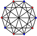
Polygons of the form _p{4}₂ are called generalized hypercubes (squares for polygons). They share vertices with the 4D p-p duoprisms, vertices connected by p-edges. Vertices are drawn in green, and p-edges are drawn in alternate colors, red and blue. The perspective is distorted slightly for odd dimensions to move overlapping vertices from the center.

• 
  ₂{4}₂, or , with 4 vertices, and 4 2-edges
• 
  ₃{4}₂, or , with 9 vertices, and 6 (triangular) 3-edges^[13]
• 
  ₄{4}₂, or , with 16 vertices, and 8 (square) 4-edges
• 
  ₅{4}₂, or , with 25 vertices, and 10 (pentagonal) 5-edges
• 
  ₆{4}₂, or , with 36 vertices, and 12 (hexagonal) 6-edges
• 
  ₇{4}₂, or , with 49 vertices, and 14 (heptagonal)7-edges
• 
  ₈{4}₂, or , with 64 vertices, and 16 (octagonal) 8-edges
• 
  ₉{4}₂, or , with 81 vertices, and 18 (enneagonal) 9-edges
• 
  ₁₀{4}₂, or , with 100 vertices, and 20 (decagonal) 10-edges

3D perspective projections of complex polygons _p{4}₂. The duals ₂{4}_p

are seen by adding vertices inside the edges, and adding edges in place of vertices.

• 
  ₃{4}₂, or with 9 vertices, 6 3-edges in 2 sets of colors
• 
  ₂{4}₃, with 6 vertices, 9 edges in 3 sets
• 
  ₄{4}₂, or with 16 vertices, 8 4-edges in 2 sets of colors and filled square 4-edges
• 
  ₅{4}₂, or with 25 vertices, 10 5-edges in 2 sets of colors

Other Complex polygons _p{r}₂

• 
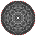
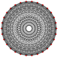
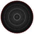
  ₃{6}₂, or , with 24 vertices in black, and 16 3-edges colored in 2 sets of 3-edges in red and blue^[14]
• 
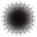
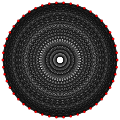
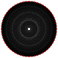
  ₃{8}₂, or , with 72 vertices in black, and 48 3-edges colored in 2 sets of 3-edges in red and blue^[15]

2D orthogonal projections of complex polygons, _p{r}_p

Polygons of the form _p{r}_p have equal number of vertices and edges. They are also self-dual.

• 
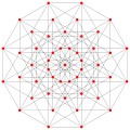
  ₃{3}₃, or , with 8 vertices in black, and 8 3-edges colored in 2 sets of 3-edges in red and blue^[16]
• 
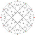
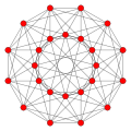
  ₃{4}₃, or , with 24 vertices and 24 3-edges shown in 3 sets of colors, one set filled^[17]
• 
  ₄{3}₄, or , with 24 vertices and 24 4-edges shown in 4 sets of colors^[17]
• 
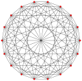
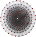
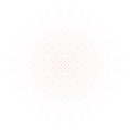
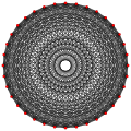
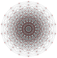
  ₃{5}₃, or , with 120 vertices and 120 3-edges^[18]
• 
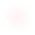
  ₅{3}₅, or , with 120 vertices and 120 5-edges^[19]

Regular complex polytopes

In general, a regular complex polytope is represented by Coxeter as _p{z₁}_q{z₂}_r{z₃}_s… or Coxeter diagram …, having symmetry _p[z₁]_q[z₂]_r[z₃]_s… or ….^[20]

There are infinite families of regular complex polytopes that occur in all dimensions, generalizing the hypercubes and cross polytopes in real space. Shephard's "generalized orthotope" generalizes the hypercube; it has symbol given by γ^p
_n = _p{4}₂{3}₂…₂{3}₂ and diagram …. Its symmetry group has diagram _p[4]₂[3]₂…₂[3]₂; in the Shephard–Todd classification, this is the group G(p, 1, n) generalizing the signed permutation matrices. Its dual regular polytope, the "generalized cross polytope", is represented by the symbol β^p
_n = ₂{3}₂{3}₂…₂{4}_p and diagram ….^[21]

A 1-dimensional regular complex polytope in ${\displaystyle \mathbb {C} ^{1}}$ is represented as , having p vertices, with its real representation a regular polygon, {p}. Coxeter also gives it symbol γ^p
₁ or β^p
₁ as 1-dimensional generalized hypercube or cross polytope. Its symmetry is _p[] or , a cyclic group of order p. In a higher polytope, _p{} or represents a p-edge element, with a 2-edge, {} or , representing an ordinary real edge between two vertices.^[21]

A dual complex polytope is constructed by exchanging k and (n-1-k)-elements of an n-polytope. For example, a dual complex polygon has vertices centered on each edge, and new edges are centered at the old vertices. A v-valence vertex creates a new v-edge, and e-edges become e-valence vertices.^[22] The dual of a regular complex polytope has a reversed symbol. Regular complex polytopes with symmetric symbols, i.e. _p{q}_p, _p{q}_r{q}_p, _p{q}_r{s}_r{q}_p, etc. are self dual.

Enumeration of regular complex polyhedra

Coxeter enumerated this list of nonstarry regular complex polyhedra in ${\displaystyle \mathbb {C} ^{3}}$, including the 5 platonic solids in ${\displaystyle \mathbb {R} ^{3}}$.^[23]

A regular complex polyhedron, _p{n₁}_q{n₂}_r or , has faces, edges, and vertex figures.

A complex regular polyhedron _p{n₁}_q{n₂}_r requires both g₁ = order(_p[n₁]_q) and g₂ = order(_q[n₂]_r) be finite.

Given g = order(_p[n₁]_q[n₂]_r), the number of vertices is g/g₂, and the number of faces is g/g₁. The number of edges is g/pr.

Space	Group	Order	Coxeter number	Polygon		Vertices	Edges		Faces		Vertex figure	Van Osspolygon	Notes
${\displaystyle \mathbb {R} ^{3}}$	G(1,1,3) 2[3]2[3]2 = [3,3]	24	4	α3 = 2{3}2{3}2 = {3,3}		4	6	{}	4	{3}	{3}	none	Real tetrahedron Same as
${\displaystyle \mathbb {R} ^{3}}$	G23 2[3]2[5]2 = [3,5]	120	10	2{3}2{5}2 = {3,5}		12	30	{}	20	{3}	{5}	none	Real icosahedron
				2{5}2{3}2 = {5,3}		20	30	{}	12	{5}	{3}	none	Real dodecahedron
${\displaystyle \mathbb {R} ^{3}}$	G(2,1,3) 2[3]2[4]2 = [3,4]	48	6	β2 3 = β3 = {3,4}		6	12	{}	8	{3}	{4}	{4}	Real octahedron Same as {}+{}+{}, order 8 Same as , order 24
${\displaystyle \mathbb {R} ^{3}}$				γ2 3 = γ3 = {4,3}		8	12	{}	6	{4}	{3}	none	Real cube Same as {}×{}×{} or
${\displaystyle \mathbb {C} ^{3}}$	G(p,1,3) 2[3]2[4]p p=2,3,4,...	6p3	3p	βp 3 = 2{3}2{4}p		3p	3p2	{}	p3	{3}	2{4}p	2{4}p	Generalized octahedron Same as p{}+p{}+p{}, order p3 Same as , order 6p2
${\displaystyle \mathbb {C} ^{3}}$				γp 3 = p{4}2{3}2		p3	3p2	p{}	3p	p{4}2	{3}	none	Generalized cube Same as p{}×p{}×p{} or
${\displaystyle \mathbb {C} ^{3}}$	G(3,1,3) 2[3]2[4]3	162	9	β3 3 = 2{3}2{4}3		9	27	{}	27	{3}	2{4}3	2{4}3	Same as 3{}+3{}+3{}, order 27 Same as , order 54
${\displaystyle \mathbb {C} ^{3}}$				γ3 3 = 3{4}2{3}2		27	27	3{}	9	3{4}2	{3}	none	Same as 3{}×3{}×3{} or
${\displaystyle \mathbb {C} ^{3}}$	G(4,1,3) 2[3]2[4]4	384	12	β4 3 = 2{3}2{4}4		12	48	{}	64	{3}	2{4}4	2{4}4	Same as 4{}+4{}+4{}, order 64 Same as , order 96
${\displaystyle \mathbb {C} ^{3}}$				γ4 3 = 4{4}2{3}2		64	48	4{}	12	4{4}2	{3}	none	Same as 4{}×4{}×4{} or
${\displaystyle \mathbb {C} ^{3}}$	G(5,1,3) 2[3]2[4]5	750	15	β5 3 = 2{3}2{4}5		15	75	{}	125	{3}	2{4}5	2{4}5	Same as 5{}+5{}+5{}, order 125 Same as , order 150
${\displaystyle \mathbb {C} ^{3}}$				γ5 3 = 5{4}2{3}2		125	75	5{}	15	5{4}2	{3}	none	Same as 5{}×5{}×5{} or
${\displaystyle \mathbb {C} ^{3}}$	G(6,1,3) 2[3]2[4]6	1296	18	β6 3 = 2{3}2{4}6		36	108	{}	216	{3}	2{4}6	2{4}6	Same as 6{}+6{}+6{}, order 216 Same as , order 216
${\displaystyle \mathbb {C} ^{3}}$				γ6 3 = 6{4}2{3}2		216	108	6{}	18	6{4}2	{3}	none	Same as 6{}×6{}×6{} or
${\displaystyle \mathbb {C} ^{3}}$	G25 3[3]3[3]3	648	9	3{3}3{3}3		27	72	3{}	27	3{3}3	3{3}3	3{4}2	Same as . ${\displaystyle \mathbb {R} ^{6}}$ representation as 221 Hessian polyhedron
	G26 2[4]3[3]3	1296	18	2{4}3{3}3		54	216	{}	72	2{4}3	3{3}3	{6}
				3{3}3{4}2		72	216	3{}	54	3{3}3	3{4}2	3{4}3	Same as [24] ${\displaystyle \mathbb {R} ^{6}}$ representation as 122

Visualizations of regular complex polyhedra

2D orthogonal projections of complex polyhedra, _p{s}_t{r}_r

• 
  Real {3,3}, or has 4 vertices, 6 edges, and 4 faces
• 
  ₃{3}₃{3}₃, or , has 27 vertices, 72 3-edges, and 27 faces, with one face highlighted blue.^[25]
• 
  ₂{4}₃{3}₃, has 54 vertices, 216 simple edges, and 72 faces, with one face highlighted blue.^[26]
• 
  ₃{3}₃{4}₂, or , has 72 vertices, 216 3-edges, and 54 vertices, with one face highlighted blue.^[27]

Generalized octahedra

Generalized octahedra have a regular construction as and quasiregular form as . All elements are simplexes.

• 
  Real {3,4}, or , with 6 vertices, 12 edges, and 8 faces
• 
  ₂{3}₂{4}₃, or , with 9 vertices, 27 edges, and 27 faces
• 
  ₂{3}₂{4}₄, or , with 12 vertices, 48 edges, and 64 faces
• 
  ₂{3}₂{4}₅, or , with 15 vertices, 75 edges, and 125 faces
• 
  ₂{3}₂{4}₆, or , with 18 vertices, 108 edges, and 216 faces
• 
  ₂{3}₂{4}₇, or , with 21 vertices, 147 edges, and 343 faces
• 
  ₂{3}₂{4}₈, or , with 24 vertices, 192 edges, and 512 faces
• 
  ₂{3}₂{4}₉, or , with 27 vertices, 243 edges, and 729 faces
• 
  ₂{3}₂{4}₁₀, or , with 30 vertices, 300 edges, and 1000 faces

Generalized cubes

Generalized cubes have a regular construction as and prismatic construction as , a product of three p-gonal 1-polytopes. Elements are lower dimensional generalized cubes.

• 
  Real {4,3}, or has 8 vertices, 12 edges, and 6 faces
• 
  ₃{4}₂{3}₂, or has 27 vertices, 27 3-edges, and 9 faces^[25]
• 
  ₄{4}₂{3}₂, or , with 64 vertices, 48 edges, and 12 faces
• 
  ₅{4}₂{3}₂, or , with 125 vertices, 75 edges, and 15 faces
• 
  ₆{4}₂{3}₂, or , with 216 vertices, 108 edges, and 18 faces
• 
  ₇{4}₂{3}₂, or , with 343 vertices, 147 edges, and 21 faces
• 
  ₈{4}₂{3}₂, or , with 512 vertices, 192 edges, and 24 faces
• 
  ₉{4}₂{3}₂, or , with 729 vertices, 243 edges, and 27 faces
• 
  ₁₀{4}₂{3}₂, or , with 1000 vertices, 300 edges, and 30 faces

Enumeration of regular complex 4-polytopes

Coxeter enumerated this list of nonstarry regular complex 4-polytopes in ${\displaystyle \mathbb {C} ^{4}}$, including the 6 convex regular 4-polytopes in ${\displaystyle \mathbb {R} ^{4}}$.^[23]

Space	Group	Order	Coxeter number	Polytope	Vertices	Edges	Faces	Cells	Van Osspolygon	Notes
${\displaystyle \mathbb {R} ^{4}}$	G(1,1,4) 2[3]2[3]2[3]2 = [3,3,3]	120	5	α4 = 2{3}2{3}2{3}2 = {3,3,3}	5	10 {}	10 {3}	5 {3,3}	none	Real 5-cell (simplex)
${\displaystyle \mathbb {R} ^{4}}$	G28 2[3]2[4]2[3]2 = [3,4,3]	1152	12	2{3}2{4}2{3}2 = {3,4,3}	24	96 {}	96 {3}	24 {3,4}	{6}	Real 24-cell
	G30 2[3]2[3]2[5]2 = [3,3,5]	14400	30	2{3}2{3}2{5}2 = {3,3,5}	120	720 {}	1200 {3}	600 {3,3}	{10}	Real 600-cell
				2{5}2{3}2{3}2 = {5,3,3}	600	1200 {}	720 {5}	120 {5,3}		Real 120-cell
${\displaystyle \mathbb {R} ^{4}}$	G(2,1,4) 2[3]2[3]2[4]p =[3,3,4]	384	8	β2 4 = β4 = {3,3,4}	8	24 {}	32 {3}	16 {3,3}	{4}	Real 16-cell Same as , order 192
${\displaystyle \mathbb {R} ^{4}}$				γ2 4 = γ4 = {4,3,3}	16	32 {}	24 {4}	8 {4,3}	none	Real tesseract Same as {}4 or , order 16
${\displaystyle \mathbb {C} ^{4}}$	G(p,1,4) 2[3]2[3]2[4]p p=2,3,4,...	24p4	4p	βp 4 = 2{3}2{3}2{4}p	4p	6p2 {}	4p3 {3}	p4 {3,3}	2{4}p	Generalized 4-orthoplex Same as , order 24p3
${\displaystyle \mathbb {C} ^{4}}$				γp 4 = p{4}2{3}2{3}2	p4	4p3 p{}	6p2 p{4}2	4p p{4}2{3}2	none	Generalized tesseract Same as p{}4 or , order p4
${\displaystyle \mathbb {C} ^{4}}$	G(3,1,4) 2[3]2[3]2[4]3	1944	12	β3 4 = 2{3}2{3}2{4}3	12	54 {}	108 {3}	81 {3,3}	2{4}3	Generalized 4-orthoplex Same as , order 648
${\displaystyle \mathbb {C} ^{4}}$				γ3 4 = 3{4}2{3}2{3}2	81	108 3{}	54 3{4}2	12 3{4}2{3}2	none	Same as 3{}4 or , order 81
${\displaystyle \mathbb {C} ^{4}}$	G(4,1,4) 2[3]2[3]2[4]4	6144	16	β4 4 = 2{3}2{3}2{4}4	16	96 {}	256 {3}	64 {3,3}	2{4}4	Same as , order 1536
${\displaystyle \mathbb {C} ^{4}}$				γ4 4 = 4{4}2{3}2{3}2	256	256 4{}	96 4{4}2	16 4{4}2{3}2	none	Same as 4{}4 or , order 256
${\displaystyle \mathbb {C} ^{4}}$	G(5,1,4) 2[3]2[3]2[4]5	15000	20	β5 4 = 2{3}2{3}2{4}5	20	150 {}	500 {3}	625 {3,3}	2{4}5	Same as , order 3000
${\displaystyle \mathbb {C} ^{4}}$				γ5 4 = 5{4}2{3}2{3}2	625	500 5{}	150 5{4}2	20 5{4}2{3}2	none	Same as 5{}4 or , order 625
${\displaystyle \mathbb {C} ^{4}}$	G(6,1,4) 2[3]2[3]2[4]6	31104	24	β6 4 = 2{3}2{3}2{4}6	24	216 {}	864 {3}	1296 {3,3}	2{4}6	Same as , order 5184
${\displaystyle \mathbb {C} ^{4}}$				γ6 4 = 6{4}2{3}2{3}2	1296	864 6{}	216 6{4}2	24 6{4}2{3}2	none	Same as 6{}4 or , order 1296
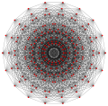
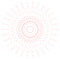
${\displaystyle \mathbb {C} ^{4}}$	G32 3[3]3[3]3[3]3	155520	30	3{3}3{3}3{3}3	240	2160 3{}	2160 3{3}3	240 3{3}3{3}3	3{4}3	Witting polytope ${\displaystyle \mathbb {R} ^{8}}$ representation as 421

Visualizations of regular complex 4-polytopes

• 
  Real {3,3,3}, , had 5 vertices, 10 edges, 10 {3} faces, and 5 {3,3} cells
• 
  Real {3,4,3}, , had 24 vertices, 96 edges, 96 {3} faces, and 24 {3,4} cells
• 
  Real {5,3,3}, , had 600 vertices, 1200 edges, 720 {5} faces, and 120 {5,3} cells
• 
  Real {3,3,5}, , had 120 vertices, 720 edges, 1200 {3} faces, and 600 {3,3} cells
• 
  Witting polytope, , has 240 vertices, 2160 3-edges, 2160 3{3}3 faces, and 240 3{3}3{3}3 cells

Generalized 4-orthoplexes

Generalized 4-orthoplexes have a regular construction as and quasiregular form as . All elements are simplexes.

• 
  Real {3,3,4}, or , with 8 vertices, 24 edges, 32 faces, and 16 cells
• 
  ₂{3}₂{3}₂{4}₃, or , with 12 vertices, 54 edges, 108 faces, and 81 cells
• 
  ₂{3}₂{3}₂{4}₄, or , with 16 vertices, 96 edges, 256 faces, and 256 cells
• 
  ₂{3}₂{3}₂{4}₅, or , with 20 vertices, 150 edges, 500 faces, and 625 cells
• 
  ₂{3}₂{3}₂{4}₆, or , with 24 vertices, 216 edges, 864 faces, and 1296 cells
• 
  ₂{3}₂{3}₂{4}₇, or , with 28 vertices, 294 edges, 1372 faces, and 2401 cells
• 
  ₂{3}₂{3}₂{4}₈, or , with 32 vertices, 384 edges, 2048 faces, and 4096 cells
• 
  ₂{3}₂{3}₂{4}₉, or , with 36 vertices, 486 edges, 2916 faces, and 6561 cells
• 
  ₂{3}₂{3}₂{4}₁₀, or , with 40 vertices, 600 edges, 4000 faces, and 10000 cells

Generalized 4-cubes

Generalized tesseracts have a regular construction as and prismatic construction as , a product of four p-gonal 1-polytopes. Elements are lower dimensional generalized cubes.

• 
  Real {4,3,3}, or , with 16 vertices, 32 edges, 24 faces, and 8 cells
• 
  ₃{4}₂{3}₂{3}₂, or , with 81 vertices, 108 edges, 54 faces, and 12 cells
• 
  ₄{4}₂{3}₂{3}₂, or , with 256 vertices, 96 edges, 96 faces, and 16 cells
• 
  ₅{4}₂{3}₂{3}₂, or , with 625 vertices, 500 edges, 150 faces, and 20 cells
• 
  ₆{4}₂{3}₂{3}₂, or , with 1296 vertices, 864 edges, 216 faces, and 24 cells
• 
  ₇{4}₂{3}₂{3}₂, or , with 2401 vertices, 1372 edges, 294 faces, and 28 cells
• 
  ₈{4}₂{3}₂{3}₂, or , with 4096 vertices, 2048 edges, 384 faces, and 32 cells
• 
  ₉{4}₂{3}₂{3}₂, or , with 6561 vertices, 2916 edges, 486 faces, and 36 cells
• 
  ₁₀{4}₂{3}₂{3}₂, or , with 10000 vertices, 4000 edges, 600 faces, and 40 cells

Enumeration of regular complex 5-polytopes

Regular complex 5-polytopes in ${\displaystyle \mathbb {C} ^{5}}$ or higher exist in three families, the real simplexes and the generalized hypercube, and orthoplex.

Space	Group	Order	Polytope	Vertices	Edges	Faces	Cells	4-faces	Van Osspolygon	Notes
${\displaystyle \mathbb {R} ^{5}}$	G(1,1,5) = [3,3,3,3]	720	α5 = {3,3,3,3}	6	15 {}	20 {3}	15 {3,3}	6 {3,3,3}	none	Real 5-simplex
${\displaystyle \mathbb {R} ^{5}}$	G(2,1,5) =[3,3,3,4]	3840	β2 5 = β5 = {3,3,3,4}	10	40 {}	80 {3}	80 {3,3}	32 {3,3,3}	{4}	Real 5-orthoplex Same as , order 1920
${\displaystyle \mathbb {R} ^{5}}$			γ2 5 = γ5 = {4,3,3,3}	32	80 {}	80 {4}	40 {4,3}	10 {4,3,3}	none	Real 5-cube Same as {}5 or , order 32
${\displaystyle \mathbb {C} ^{5}}$	G(p,1,5) 2[3]2[3]2[3]2[4]p	120p5	βp 5 = 2{3}2{3}2{3}2{4}p	5p	10p2 {}	10p3 {3}	5p4 {3,3}	p5 {3,3,3}	2{4}p	Generalized 5-orthoplex Same as , order 120p4
${\displaystyle \mathbb {C} ^{5}}$			γp 5 = p{4}2{3}2{3}2{3}2	p5	5p4 p{}	10p3 p{4}2	10p2 p{4}2{3}2	5p p{4}2{3}2{3}2	none	Generalized 5-cube Same as p{}5 or , order p5
${\displaystyle \mathbb {C} ^{5}}$	G(3,1,5) 2[3]2[3]2[3]2[4]3	29160	β3 5 = 2{3}2{3}2{3}2{4}3	15	90 {}	270 {3}	405 {3,3}	243 {3,3,3}	2{4}3	Same as , order 9720
${\displaystyle \mathbb {C} ^{5}}$			γ3 5 = 3{4}2{3}2{3}2{3}2	243	405 3{}	270 3{4}2	90 3{4}2{3}2	15 3{4}2{3}2{3}2	none	Same as 3{}5 or , order 243
${\displaystyle \mathbb {C} ^{5}}$	G(4,1,5) 2[3]2[3]2[3]2[4]4	122880	β4 5 = 2{3}2{3}2{3}2{4}4	20	160 {}	640 {3}	1280 {3,3}	1024 {3,3,3}	2{4}4	Same as , order 30720
${\displaystyle \mathbb {C} ^{5}}$			γ4 5 = 4{4}2{3}2{3}2{3}2	1024	1280 4{}	640 4{4}2	160 4{4}2{3}2	20 4{4}2{3}2{3}2	none	Same as 4{}5 or , order 1024
${\displaystyle \mathbb {C} ^{5}}$	G(5,1,5) 2[3]2[3]2[3]2[4]5	375000	β5 5 = 2{3}2{3}2{3}2{5}5	25	250 {}	1250 {3}	3125 {3,3}	3125 {3,3,3}	2{5}5	Same as , order 75000
${\displaystyle \mathbb {C} ^{5}}$			γ5 5 = 5{4}2{3}2{3}2{3}2	3125	3125 5{}	1250 5{5}2	250 5{5}2{3}2	25 5{4}2{3}2{3}2	none	Same as 5{}5 or , order 3125
${\displaystyle \mathbb {C} ^{5}}$	G(6,1,5) 2[3]2[3]2[3]2[4]6	933210	β6 5 = 2{3}2{3}2{3}2{4}6	30	360 {}	2160 {3}	6480 {3,3}	7776 {3,3,3}	2{4}6	Same as , order 155520
${\displaystyle \mathbb {C} ^{5}}$			γ6 5 = 6{4}2{3}2{3}2{3}2	7776	6480 6{}	2160 6{4}2	360 6{4}2{3}2	30 6{4}2{3}2{3}2	none	Same as 6{}5 or , order 7776

Visualizations of regular complex 5-polytopes

Generalized 5-orthoplexes

Generalized 5-orthoplexes have a regular construction as and quasiregular form as . All elements are simplexes.

• 
  Real {3,3,3,4}, , with 10 vertices, 40 edges, 80 faces, 80 cells, and 32 4-faces
• 
  ₂{3}₂{3}₂{3}₂{4}₃, , with 15 vertices, 90 edges, 270 faces, 405 cells, and 243 4-faces
• 
  ₂{3}₂{3}₂{3}₂{4}₄, , with 20 vertices, 160 edges, 640 faces, 1280 cells, and 1024 4-faces
• 
  ₂{3}₂{3}₂{3}₂{4}₅, , with 25 vertices, 250 edges, 1250 faces, 3125 cells, and 3125 4-faces
• 
  ₂{3}₂{3}₂{3}₂{4}₆, , with 30 vertices, 360 edges, 2160 faces, 6480 cells, 7776 4-faces
• 
  ₂{3}₂{3}₂{3}₂{4}₇, , with 35 vertices, 490 edges, 3430 faces, 12005 cells, 16807 4-faces
• 
  ₂{3}₂{3}₂{3}₂{4}₈, , with 40 vertices, 640 edges, 5120 faces, 20480 cells, 32768 4-faces
• 
  ₂{3}₂{3}₂{3}₂{4}₉, , with 45 vertices, 810 edges, 7290 faces, 32805 cells, 59049 4-faces
• 
  ₂{3}₂{3}₂{3}₂{4}₁₀, , with 50 vertices, 1000 edges, 10000 faces, 50000 cells, 100000 4-faces

Generalized 5-cubes

Generalized 5-cubes have a regular construction as and prismatic construction as , a product of five p-gonal 1-polytopes. Elements are lower dimensional generalized cubes.

• 
  Real {4,3,3,3}, , with 32 vertices, 80 edges, 80 faces, 40 cells, and 10 4-faces
• 
  ₃{4}₂{3}₂{3}₂{3}₂, , with 243 vertices, 405 edges, 270 faces, 90 cells, and 15 4-faces
• 
  ₄{4}₂{3}₂{3}₂{3}₂, , with 1024 vertices, 1280 edges, 640 faces, 160 cells, and 20 4-faces
• 
  ₅{4}₂{3}₂{3}₂{3}₂, , with 3125 vertices, 3125 edges, 1250 faces, 250 cells, and 25 4-faces
• 
  ₆{4}₂{3}₂{3}₂{3}₂, , with 7776 vertices, 6480 edges, 2160 faces, 360 cells, and 30 4-faces

Enumeration of regular complex 6-polytopes

Space	Group	Order	Polytope	Vertices	Edges	Faces	Cells	4-faces	5-faces	Van Osspolygon	Notes
${\displaystyle \mathbb {R} ^{6}}$	G(1,1,6) = [3,3,3,3,3]	720	α6 = {3,3,3,3,3}	7	21 {}	35 {3}	35 {3,3}	21 {3,3,3}	7 {3,3,3,3}	none	Real 6-simplex
${\displaystyle \mathbb {R} ^{6}}$	G(2,1,6) [3,3,3,4]	46080	β2 6 = β6 = {3,3,3,4}	12	60 {}	160 {3}	240 {3,3}	192 {3,3,3}	64 {3,3,3,3}	{4}	Real 6-orthoplex Same as , order 23040
${\displaystyle \mathbb {R} ^{6}}$			γ2 6 = γ6 = {4,3,3,3}	64	192 {}	240 {4}	160 {4,3}	60 {4,3,3}	12 {4,3,3,3}	none	Real 6-cube Same as {}6 or , order 64
${\displaystyle \mathbb {C} ^{6}}$	G(p,1,6) 2[3]2[3]2[3]2[4]p	720p6	βp 6 = 2{3}2{3}2{3}2{4}p	6p	15p2 {}	20p3 {3}	15p4 {3,3}	6p5 {3,3,3}	p6 {3,3,3,3}	2{4}p	Generalized 6-orthoplex Same as , order 720p5
${\displaystyle \mathbb {C} ^{6}}$			γp 6 = p{4}2{3}2{3}2{3}2	p6	6p5 p{}	15p4 p{4}2	20p3 p{4}2{3}2	15p2 p{4}2{3}2{3}2	6p p{4}2{3}2{3}2{3}2	none	Generalized 6-cube Same as p{}6 or , order p6

Visualizations of regular complex 6-polytopes

Generalized 6-orthoplexes

Generalized 6-orthoplexes have a regular construction as and quasiregular form as . All elements are simplexes.

• 
  Real {3,3,3,3,4}, , with 12 vertices, 60 edges, 160 faces, 240 cells, 192 4-faces, and 64 5-faces
• 
  ₂{3}₂{3}₂{3}₂{3}₂{4}₃, , with 18 vertices, 135 edges, 540 faces, 1215 cells, 1458 4-faces, and 729 5-faces
• 
  ₂{3}₂{3}₂{3}₂{3}₂{4}₄, , with 24 vertices, 240 edges, 1280 faces, 3840 cells, 6144 4-faces, and 4096 5-faces
• 
  ₂{3}₂{3}₂{3}₂{3}₂{4}₅, , with 30 vertices, 375 edges, 2500 faces, 9375 cells, 18750 4-faces, and 15625 5-faces
• 
  ₂{3}₂{3}₂{3}₂{3}₂{4}₆, , with 36 vertices, 540 edges, 4320 faces, 19440 cells, 46656 4-faces, and 46656 5-faces
• 
  ₂{3}₂{3}₂{3}₂{3}₂{4}₇, , with 42 vertices, 735 edges, 6860 faces, 36015 cells, 100842 4-faces, 117649 5-faces
• 
  ₂{3}₂{3}₂{3}₂{3}₂{4}₈, , with 48 vertices, 960 edges, 10240 faces, 61440 cells, 196608 4-faces, 262144 5-faces
• 
  ₂{3}₂{3}₂{3}₂{3}₂{4}₉, , with 54 vertices, 1215 edges, 14580 faces, 98415 cells, 354294 4-faces, 531441 5-faces
• 
  ₂{3}₂{3}₂{3}₂{3}₂{4}₁₀, , with 60 vertices, 1500 edges, 20000 faces, 150000 cells, 600000 4-faces, 1000000 5-faces

Generalized 6-cubes

Generalized 6-cubes have a regular construction as and prismatic construction as , a product of six p-gonal 1-polytopes. Elements are lower dimensional generalized cubes.

• 
  Real {3,3,3,3,3,4}, , with 64 vertices, 192 edges, 240 faces, 160 cells, 60 4-faces, and 12 5-faces
• 
  ₃{4}₂{3}₂{3}₂{3}₂{3}₂, , with 729 vertices, 1458 edges, 1215 faces, 540 cells, 135 4-faces, and 18 5-faces
• 
  ₄{4}₂{3}₂{3}₂{3}₂{3}₂, , with 4096 vertices, 6144 edges, 3840 faces, 1280 cells, 240 4-faces, and 24 5-faces
• 
  ₅{4}₂{3}₂{3}₂{3}₂{3}₂, , with 15625 vertices, 18750 edges, 9375 faces, 2500 cells, 375 4-faces, and 30 5-faces

Enumeration of regular complex apeirotopes

Coxeter enumerated this list of nonstarry regular complex apeirotopes or honeycombs.^[28]

For each dimension there are 12 apeirotopes symbolized as δ^p,r
_n+1 exists in any dimensions ${\displaystyle \mathbb {C} ^{n}}$, or ${\displaystyle \mathbb {R} ^{n}}$ if p=q=2. Coxeter calls these generalized cubic honeycombs for n>2.^[29]

Each has proportional element counts given as:

k-faces = ${\displaystyle {n \choose k}p^{n-k}r^{k}}$, where ${\displaystyle {n \choose m}={\frac {n!}{m!\,(n-m)!}}}$ and n! denotes the factorial of n.

Regular complex 1-polytopes

The only regular complex 1-polytope is _∞{}, or . Its real representation is an apeirogon, {∞}, or .

Regular complex apeirogons

Rank 2 complex apeirogons have symmetry _p[q]_r, where 1/p + 2/q + 1/r = 1. Coxeter expresses them as δ^p,r
₂ where q is constrained to satisfy q = 2/(1 – (p + r)/pr).^[30]

There are 8 solutions:

2[∞]2	3[12]2	4[8]2	6[6]2	3[6]3	6[4]3	4[4]4	6[3]6

There are two excluded solutions odd q and unequal p and r: ₁₀[5]₂ and ₁₂[3]₄, or and .

A regular complex apeirogon _p{q}_r has p-edges and r-gonal vertex figures. The dual apeirogon of _p{q}_r is _r{q}_p. An apeirogon of the form _p{q}_p is self-dual. Groups of the form _p[2q]₂ have a half symmetry _p[q]_p, so a regular apeirogon is the same as quasiregular .^[31]

Apeirogons can be represented on the Argand plane share four different vertex arrangements. Apeirogons of the form ₂{q}_r have a vertex arrangement as {q/2,p}. The form _p{q}₂ have vertex arrangement as r{p,q/2}. Apeirogons of the form _p{4}_r have vertex arrangements {p,r}.

Including affine nodes, and ${\displaystyle \mathbb {C} ^{2}}$, there are 3 more infinite solutions: _∞[2]_∞, _∞[4]₂, _∞[3]₃, and , , and . The first is an index 2 subgroup of the second. The vertices of these apeirogons exist in ${\displaystyle \mathbb {C} ^{1}}$.

Rank 2

Space	Group	Apeirogon		Edge	${\displaystyle \mathbb {R} ^{2}}$ rep.[32]	Picture	Notes
${\displaystyle \mathbb {R} ^{1}}$	2[∞]2 = [∞]	δ2,2 2 = {∞}		{}			Real apeirogon Same as
${\displaystyle \mathbb {C} ^{2}}$ / ${\displaystyle \mathbb {C} ^{1}}$	∞[4]2	∞{4}2		∞{}	{4,4}		Same as
${\displaystyle \mathbb {C} ^{1}}$	∞[3]3	∞{3}3		∞{}	{3,6}		Same as
${\displaystyle \mathbb {C} ^{1}}$	p[q]r	δp,r 2 = p{q}r		p{}
${\displaystyle \mathbb {C} ^{1}}$	3[12]2	δ3,2 2 = 3{12}2		3{}	r{3,6}		Same as
		δ2,3 2 = 2{12}3		{}	{6,3}
${\displaystyle \mathbb {C} ^{1}}$	3[6]3	δ3,3 2 = 3{6}3		3{}	{3,6}		Same as
${\displaystyle \mathbb {C} ^{1}}$	4[8]2	δ4,2 2 = 4{8}2		4{}	{4,4}		Same as
		δ2,4 2 = 2{8}4		{}	{4,4}
${\displaystyle \mathbb {C} ^{1}}$	4[4]4	δ4,4 2 = 4{4}4		4{}	{4,4}		Same as
${\displaystyle \mathbb {C} ^{1}}$	6[6]2	δ6,2 2 = 6{6}2		6{}	r{3,6}		Same as
		δ2,6 2 = 2{6}6		{}	{3,6}
${\displaystyle \mathbb {C} ^{1}}$	6[4]3	δ6,3 2 = 6{4}3		6{}	{6,3}
		δ3,6 2 = 3{4}6		3{}	{3,6}
${\displaystyle \mathbb {C} ^{1}}$	6[3]6	δ6,6 2 = 6{3}6		6{}	{3,6}		Same as

Regular complex apeirohedra

There are 22 regular complex apeirohedra, of the form _p{a}_q{b}_r. 8 are self-dual (p=r and a=b), while 14 exist as dual polytope pairs. Three are entirely real (p=q=r=2).

Coxeter symbolizes 12 of them as δ^p,r
₃ or _p{4}₂{4}_r is the regular form of the product apeirotope δ^p,r
₂ × δ^p,r
₂ or _p{q}_r × _p{q}_r, where q is determined from p and r.

is the same as , as well as , for p,r=2,3,4,6. Also = .^[33]

Rank 3

Space	Group	Apeirohedron		Vertex	Edge		Face		van Oss apeirogon	Notes
${\displaystyle \mathbb {C} ^{3}}$	2[3]2[4]∞	∞{4}2{3}2				∞{}		∞{4}2		Same as ∞{}×∞{}×∞{} or Real representation {4,3,4}
${\displaystyle \mathbb {C} ^{2}}$	p[4]2[4]r	p{4}2{4}r		p2	2pr	p{}	r2	p{4}2	2{q}r	Same as , p,r=2,3,4,6
${\displaystyle \mathbb {R} ^{2}}$	[4,4]	δ2,2 3 = {4,4}		4	8	{}	4	{4}	{∞}	Real square tiling Same as or or
${\displaystyle \mathbb {C} ^{2}}$	3[4]2[4]2   3[4]2[4]3 4[4]2[4]2   4[4]2[4]4 6[4]2[4]2   6[4]2[4]3   6[4]2[4]6	3{4}2{4}2 2{4}2{4}3 3{4}2{4}3 4{4}2{4}2 2{4}2{4}4 4{4}2{4}4 6{4}2{4}2 2{4}2{4}6 6{4}2{4}3 3{4}2{4}6 6{4}2{4}6		9 4 9 16 4 16 36 4 36 9 36	12 12 18 16 16 32 24 24 36 36 72	3{} {} 3{} 4{} {} 4{} 6{} {} 6{} 3{} 6{}	4 9 9 4 16 16 4 36 9 36 36	3{4}2 {4} 3{4}2 4{4}2 {4} 4{4}2 6{4}2 {4} 6{4}2 3{4}2 6{4}2	p{q}r	Same as or or Same as Same as Same as or or Same as Same as Same as or or Same as Same as Same as Same as

Space	Group	Apeirohedron		Vertex	Edge		Face		van Oss apeirogon	Notes
${\displaystyle \mathbb {C} ^{2}}$	2[4]r[4]2	2{4}r{4}2		2		{}	2	p{4}2'	2{4}r	Same as and , r=2,3,4,6
${\displaystyle \mathbb {R} ^{2}}$	[4,4]	{4,4}		2	4	{}	2	{4}	{∞}	Same as and
${\displaystyle \mathbb {C} ^{2}}$	2[4]3[4]2 2[4]4[4]2 2[4]6[4]2	2{4}3{4}2 2{4}4{4}2 2{4}6{4}2		2	9 16 36	{}	2	2{4}3 2{4}4 2{4}6	2{q}r	Same as and Same as and Same as and [34]

Space	Group	Apeirohedron		Vertex	Edge		Face		van Oss apeirogon	Notes
${\displaystyle \mathbb {R} ^{2}}$	2[6]2[3]2 = [6,3]	{3,6}		1	3	{}	2	{3}	{∞}	Real triangular tiling
		{6,3}		2	3	{}	1	{6}	none	Real hexagonal tiling
${\displaystyle \mathbb {C} ^{2}}$	3[4]3[3]3	3{3}3{4}3		1	8	3{}	3	3{3}3	3{4}6	Same as
		3{4}3{3}3		3	8	3{}	1	3{4}3	3{12}2
${\displaystyle \mathbb {C} ^{2}}$	4[3]4[3]4	4{3}4{3}4		1	6	4{}	1	4{3}4	4{4}4	Self-dual, same as
${\displaystyle \mathbb {C} ^{2}}$	4[3]4[4]2	4{3}4{4}2		1	12	4{}	3	4{3}4	2{8}4	Same as
		2{4}4{3}4		3	12	{}	1	2{4}4	4{4}4

Regular complex 3-apeirotopes

There are 16 regular complex apeirotopes in ${\displaystyle \mathbb {C} ^{3}}$. Coxeter expresses 12 of them by δ^p,r
₃ where q is constrained to satisfy q = 2/(1 – (p + r)/pr). These can also be decomposed as product apeirotopes: = . The first case is the ${\displaystyle \mathbb {R} ^{3}}$ cubic honeycomb.

Rank 4

Space	Group	3-apeirotope	Vertex	Edge	Face	Cell	van Oss apeirogon	Notes
${\displaystyle \mathbb {C} ^{3}}$	p[4]2[3]2[4]r	δp,r 3 = p{4}2{3}2{4}r		p{}	p{4}2	p{4}2{3}2	p{q}r	Same as
${\displaystyle \mathbb {R} ^{3}}$	2[4]2[3]2[4]2 =[4,3,4]	δ2,2 3 = 2{4}2{3}2{4}2		{}	{4}	{4,3}		Cubic honeycomb Same as or or
${\displaystyle \mathbb {C} ^{3}}$	3[4]2[3]2[4]2	δ3,2 3 = 3{4}2{3}2{4}2		3{}	3{4}2	3{4}2{3}2		Same as or or
		δ2,3 3 = 2{4}2{3}2{4}3		{}	{4}	{4,3}		Same as
${\displaystyle \mathbb {C} ^{3}}$	3[4]2[3]2[4]3	δ3,3 3 = 3{4}2{3}2{4}3		3{}	3{4}2	3{4}2{3}2		Same as
${\displaystyle \mathbb {C} ^{3}}$	4[4]2[3]2[4]2	δ4,2 3 = 4{4}2{3}2{4}2		4{}	4{4}2	4{4}2{3}2		Same as or or
		δ2,4 3 = 2{4}2{3}2{4}4		{}	{4}	{4,3}		Same as
${\displaystyle \mathbb {C} ^{3}}$	4[4]2[3]2[4]4	δ4,4 3 = 4{4}2{3}2{4}4		4{}	4{4}2	4{4}2{3}2		Same as
${\displaystyle \mathbb {C} ^{3}}$	6[4]2[3]2[4]2	δ6,2 3 = 6{4}2{3}2{4}2		6{}	6{4}2	6{4}2{3}2		Same as or or
		δ2,6 3 = 2{4}2{3}2{4}6		{}	{4}	{4,3}		Same as
${\displaystyle \mathbb {C} ^{3}}$	6[4]2[3]2[4]3	δ6,3 3 = 6{4}2{3}2{4}3		6{}	6{4}2	6{4}2{3}2		Same as
		δ3,6 3 = 3{4}2{3}2{4}6		3{}	3{4}2	3{4}2{3}2		Same as
${\displaystyle \mathbb {C} ^{3}}$	6[4]2[3]2[4]6	δ6,6 3 = 6{4}2{3}2{4}6		6{}	6{4}2	6{4}2{3}2		Same as

Rank 4, exceptional cases

Space	Group	3-apeirotope	Vertex	Edge	Face	Cell	van Oss apeirogon	Notes
${\displaystyle \mathbb {C} ^{3}}$	2[4]3[3]3[3]3	3{3}3{3}3{4}2	1	24 3{}	27 3{3}3	2 3{3}3{3}3	3{4}6	Same as
		2{4}3{3}3{3}3	2	27 {}	24 2{4}3	1 2{4}3{3}3	2{12}3
${\displaystyle \mathbb {C} ^{3}}$	2[3]2[4]3[3]3	2{3}2{4}3{3}3	1	27 {}	72 2{3}2	8 2{3}2{4}3	2{6}6
		3{3}3{4}2{3}2	8	72 3{}	27 3{3}3	1 3{3}3{4}2	3{6}3	Same as or

Regular complex 4-apeirotopes

There are 15 regular complex apeirotopes in ${\displaystyle \mathbb {C} ^{4}}$. Coxeter expresses 12 of them by δ^p,r
₄ where q is constrained to satisfy q = 2/(1 – (p + r)/pr). These can also be decomposed as product apeirotopes: = . The first case is the ${\displaystyle \mathbb {R} ^{4}}$ tesseractic honeycomb. The 16-cell honeycomb and 24-cell honeycomb are real solutions. The last solution is generated has Witting polytope elements.

Rank 5

Space	Group	4-apeirotope	Vertex	Edge	Face	Cell	4-face	van Oss apeirogon	Notes
${\displaystyle \mathbb {C} ^{4}}$	p[4]2[3]2[3]2[4]r	δp,r 4 = p{4}2{3}2{3}2{4}r		p{}	p{4}2	p{4}2{3}2	p{4}2{3}2{3}2	p{q}r	Same as
${\displaystyle \mathbb {R} ^{4}}$	2[4]2[3]2[3]2[4]2	δ2,2 4 = {4,3,3,3}		{}	{4}	{4,3}	{4,3,3}	{∞}	Tesseractic honeycomb Same as
${\displaystyle \mathbb {R} ^{4}}$	2[3]2[4]2[3]2[3]2 =[3,4,3,3]	{3,3,4,3}	1	12 {}	32 {3}	24 {3,3}	3 {3,3,4}		Real 16-cell honeycomb Same as
		{3,4,3,3}	3	24 {}	32 {3}	12 {3,4}	1 {3,4,3}		Real 24-cell honeycomb Same as or
${\displaystyle \mathbb {C} ^{4}}$	3[3]3[3]3[3]3[3]3	3{3}3{3}3{3}3{3}3	1	80 3{}	270 3{3}3	80 3{3}3{3}3	1 3{3}3{3}3{3}3	3{4}6	${\displaystyle \mathbb {R} ^{8}}$ representation 521

Regular complex 5-apeirotopes and higher

There are only 12 regular complex apeirotopes in ${\displaystyle \mathbb {C} ^{5}}$ or higher,^[35] expressed δ^p,r
_n where q is constrained to satisfy q = 2/(1 – (p + r)/pr). These can also be decomposed a product of n apeirogons: ... = ... . The first case is the real ${\displaystyle \mathbb {R} ^{n}}$ hypercube honeycomb.

Rank 6

Space	Group	5-apeirotopes	Vertices	Edge	Face	Cell	4-face	5-face	van Oss apeirogon	Notes
${\displaystyle \mathbb {C} ^{5}}$	p[4]2[3]2[3]2[3]2[4]r	δp,r 5 = p{4}2{3}2{3}2{3}2{4}r		p{}	p{4}2	p{4}2{3}2	p{4}2{3}2{3}2	p{4}2{3}2{3}2{3}2	p{q}r	Same as
${\displaystyle \mathbb {R} ^{5}}$	2[4]2[3]2[3]2[3]2[4]2 =[4,3,3,3,4]	δ2,2 5 = {4,3,3,3,4}		{}	{4}	{4,3}	{4,3,3}	{4,3,3,3}	{∞}	5-cubic honeycomb Same as

van Oss polygon

A van Oss polygon is a regular polygon in the plane (real plane ${\displaystyle \mathbb {R} ^{2}}$, or unitary plane ${\displaystyle \mathbb {C} ^{2}}$) in which both an edge and the centroid of a regular polytope lie, and formed of elements of the polytope. Not all regular polytopes have Van Oss polygons.

For example, the van Oss polygons of a real octahedron are the three squares whose planes pass through its center. In contrast a cube does not have a van Oss polygon because the edge-to-center plane cuts diagonally across two square faces and the two edges of the cube which lie in the plane do not form a polygon.

Infinite honeycombs also have van Oss apeirogons. For example, the real square tiling and triangular tiling have apeirogons {∞} van Oss apeirogons.^[36]

If it exists, the van Oss polygon of regular complex polytope of the form _p{q}_r{s}_t... has p-edges.

Non-regular complex polytopes

Product complex polytopes

Example product complex polytope

Complex product polygon or {}×5{} has 10 vertices connected by 5 2-edges and 2 5-edges, with its real representation as a 3-dimensional pentagonal prism.

The dual polygon,{}+5{} has 7 vertices centered on the edges of the original, connected by 10 edges. Its real representation is a pentagonal bipyramid.

Some complex polytopes can be represented as Cartesian products. These product polytopes are not strictly regular since they'll have more than one facet type, but some can represent lower symmetry of regular forms if all the orthogonal polytopes are identical. For example, the product _p{}×_p{} or of two 1-dimensional polytopes is the same as the regular _p{4}₂ or . More general products, like _p{}×_q{} have real representations as the 4-dimensional p-q duoprisms. The dual of a product polytope can be written as a sum _p{}+_q{} and have real representations as the 4-dimensional p-q duopyramid. The _p{}+_p{} can have its symmetry doubled as a regular complex polytope ₂{4}_p or .

Similarly, a ${\displaystyle \mathbb {C} ^{3}}$ complex polyhedron can be constructed as a triple product: _p{}×_p{}×_p{} or is the same as the regular generalized cube, _p{4}₂{3}₂ or , as well as product _p{4}₂×_p{} or .^[37]

Quasiregular polygons

A quasiregular polygon is a truncation of a regular polygon. A quasiregular polygon contains alternate edges of the regular polygons and . The quasiregular polygon has p vertices on the p-edges of the regular form.

Example quasiregular polygons

p[q]r	2[4]2	3[4]2	4[4]2	5[4]2	6[4]2	7[4]2	8[4]2	3[3]3	3[4]3
Regular	4 2-edges	9 3-edges	16 4-edges	25 5-edges	36 6-edges	49 8-edges	64 8-edges
Quasiregular	= 4+4 2-edges	6 2-edges 9 3-edges	8 2-edges 16 4-edges	10 2-edges 25 5-edges	12 2-edges 36 6-edges	14 2-edges 49 7-edges	16 2-edges 64 8-edges	=	=
Regular	4 2-edges	6 2-edges	8 2-edges	10 2-edges	12 2-edges	14 2-edges	16 2-edges

Quasiregular apeirogons

There are 7 quasiregular complex apeirogons which alternate edges of a regular apeirogon and its regular dual. The vertex arrangements of these apeirogon have real representations with the regular and uniform tilings of the Euclidean plane. The last column for the 6{3}6 apeirogon is not only self-dual, but the dual coincides with itself with overlapping hexagonal edges, thus their quasiregular form also has overlapping hexagonal edges, so it can't be drawn with two alternating colors like the others. The symmetry of the self-dual families can be doubled, so creating an identical geometry as the regular forms: =

p[q]r	4[8]2	4[4]4	6[6]2	6[4]3	3[12]2	3[6]3	6[3]6
Regular or p{q}r
Quasiregular		=				=	=
Regular dual or r{q}p

Quasiregular polyhedra

Like real polytopes, a complex quasiregular polyhedron can be constructed as a rectification (a complete truncation) of a regular polyhedron. Vertices are created mid-edge of the regular polyhedron and faces of the regular polyhedron and its dual are positioned alternating across common edges.

For example, a p-generalized cube, , has p³ vertices, 3p² edges, and 3p p-generalized square faces, while the p-generalized octahedron, , has 3p vertices, 3p² edges and p³ triangular faces. The middle quasiregular form p-generalized cuboctahedron, , has 3p² vertices, 3p³ edges, and 3p+p³ faces.

Also the rectification of the Hessian polyhedron , is , a quasiregular form sharing the geometry of the regular complex polyhedron .

Quasiregular examples

Generalized cube/octahedra						Hessian polyhedron
	p=2 (real)	p=3	p=4	p=5	p=6
Generalized cubes (regular)	Cube , 8 vertices, 12 2-edges, and 6 faces.	, 27 vertices, 27 3-edges, and 9 faces, with one face blue and red	, 64 vertices, 48 4-edges, and 12 faces.	, 125 vertices, 75 5-edges, and 15 faces.	, 216 vertices, 108 6-edges, and 18 faces.	, 27 vertices, 72 6-edges, and 27 faces.
Generalized cuboctahedra (quasiregular)	Cuboctahedron , 12 vertices, 24 2-edges, and 6+8 faces.	, 27 vertices, 81 2-edges, and 9+27 faces, with one face blue	, 48 vertices, 192 2-edges, and 12+64 faces, with one face blue	, 75 vertices, 375 2-edges, and 15+125 faces.	, 108 vertices, 648 2-edges, and 18+216 faces.	= , 72 vertices, 216 3-edges, and 54 faces.
Generalized octahedra (regular)	Octahedron , 6 vertices, 12 2-edges, and 8 {3} faces.	, 9 vertices, 27 2-edges, and 27 {3} faces.	, 12 vertices, 48 2-edges, and 64 {3} faces.	, 15 vertices, 75 2-edges, and 125 {3} faces.	, 18 vertices, 108 2-edges, and 216 {3} faces.	, 27 vertices, 72 6-edges, and 27 faces.

Other complex polytopes with unitary reflections of period two

Other nonregular complex polytopes can be constructed within unitary reflection groups that don't make linear Coxeter graphs. In Coxeter diagrams with loops Coxeter marks a special period interior, like or symbol (1₁ 1 1)³, and group [1 1 1]³.^[38][39] These complex polytopes have not been systematically explored beyond a few cases.

The group is defined by 3 unitary reflections, R₁, R₂, R₃, all order 2: R₁² = R₁² = R₃² = (R₁R₂)³ = (R₂R₃)³ = (R₃R₁)³ = (R₁R₂R₃R₁)^p = 1. The period p can be seen as a double rotation in real ${\displaystyle \mathbb {R} ^{4}}$.

As with all Wythoff constructions, polytopes generated by reflections, the number of vertices of a single-ringed Coxeter diagram polytope is equal to the order of the group divided by the order of the subgroup where the ringed node is removed. For example, a real cube has Coxeter diagram , with octahedral symmetry order 48, and subgroup dihedral symmetry order 6, so the number of vertices of a cube is 48/6=8. Facets are constructed by removing one node furthest from the ringed node, for example for the cube. Vertex figures are generated by removing a ringed node and ringing one or more connected nodes, and for the cube.

Coxeter represents these groups by the following symbols. Some groups have the same order, but a different structure, defining the same vertex arrangement in complex polytopes, but different edges and higher elements, like and with p≠3.^[40]

Groups generated by unitary reflections

Coxeter diagram	Order	Symbol or Position in Table VII of Shephard and Todd (1954)
, ( and ), , ...	pn − 1 n!, p ≥ 3	G(p, p, n), [p], [1 1 1]p, [1 1 (n−2)p]3
,	72·6!, 108·9!	Nos. 33, 34, [1 2 2]3, [1 2 3]3
, ( and ), ( and )	14·4!, 3·6!, 64·5!	Nos. 24, 27, 29

Coxeter calls some of these complex polyhedra almost regular because they have regular facets and vertex figures. The first is a lower symmetry form of the generalized cross-polytope in ${\displaystyle \mathbb {C} ^{3}}$. The second is a fractional generalized cube, reducing p-edges into single vertices leaving ordinary 2-edges. Three of them are related to the finite regular skew polyhedron in ${\displaystyle \mathbb {R} ^{4}}$.

Some almost regular complex polyhedra^[41]

Space	Group	Order	Coxeter symbols	Vertices	Edges	Faces	Vertex figure	Notes
${\displaystyle \mathbb {C} ^{3}}$	[1 1 1p]3 p=2,3,4...	6p2	(1 1 11p)3	3p	3p2	{3}	{2p}	Shephard symbol (1 1; 11)p same as βp 3 =
			(11 1 1p)3	p2		{3}	{6}	Shephard symbol (11 1; 1)p 1/p γp 3
${\displaystyle \mathbb {R} ^{3}}$	[1 1 12]3	24	(1 1 112)3	6	12	8 {3}	{4}	Same as β2 3 = = real octahedron
			(11 1 12)3	4	6	4 {3}	{3}	1/2 γ2 3 = = α3 = real tetrahedron
${\displaystyle \mathbb {C} ^{3}}$	[1 1 1]3	54	(1 1 11)3	9	27	{3}	{6}	Shephard symbol (1 1; 11)3 same as β3 3 =
			(11 1 1)3	9	27	{3}	{6}	Shephard symbol (11 1; 1)3 1/3 γ3 3 = β3 3
${\displaystyle \mathbb {C} ^{3}}$	[1 1 14]3	96	(1 1 114)3	12	48	{3}	{8}	Shephard symbol (1 1; 11)4 same as β4 3 =
			(11 1 14)3	16		{3}	{6}	Shephard symbol (11 1; 1)4 1/4 γ4 3
${\displaystyle \mathbb {C} ^{3}}$	[1 1 15]3	150	(1 1 115)3	15	75	{3}	{10}	Shephard symbol (1 1; 11)5 same as β5 3 =
			(11 1 15)3	25		{3}	{6}	Shephard symbol (11 1; 1)5 1/5 γ5 3
${\displaystyle \mathbb {C} ^{3}}$	[1 1 16]3	216	(1 1 116)3	18	216	{3}	{12}	Shephard symbol (1 1; 11)6 same as β6 3 =
			(11 1 16)3	36		{3}	{6}	Shephard symbol (11 1; 1)6 1/6 γ6 3
${\displaystyle \mathbb {C} ^{3}}$	[1 1 14]4	336	(1 1 114)4	42	168	112 {3}	{8}	${\displaystyle \mathbb {R} ^{4}}$ representation {3,8|,4} = {3,8}8
			(11 1 14)4	56		{3}	{6}
${\displaystyle \mathbb {C} ^{3}}$	[1 1 15]4	2160	(1 1 115)4	216	1080	720 {3}	{10}	${\displaystyle \mathbb {R} ^{4}}$ representation {3,10|,4} = {3,10}8
			(11 1 15)4	360		{3}	{6}
${\displaystyle \mathbb {C} ^{3}}$	[1 1 14]5		(1 1 114)5	270	1080	720 {3}	{8}	${\displaystyle \mathbb {R} ^{4}}$ representation {3,8|,5} = {3,8}10
			(11 1 14)5	360		{3}	{6}

Coxeter defines other groups with anti-unitary constructions, for example these three. The first was discovered and drawn by Peter McMullen in 1966.^[42]

More almost regular complex polyhedra^[41]

Space	Group	Order	Coxeter symbols	Vertices	Edges	Faces	Vertex figure	Notes
${\displaystyle \mathbb {C} ^{3}}$	[1 14 14](3)	336	(11 14 14)(3)	56	168	84 {4}	{6}	${\displaystyle \mathbb {R} ^{4}}$ representation {4,6|,3} = {4,6}6
${\displaystyle \mathbb {C} ^{3}}$	[15 14 14](3)	2160	(115 14 14)(3)	216	1080	540 {4}	{10}	${\displaystyle \mathbb {R} ^{4}}$ representation {4,10|,3} = {4,10}6
${\displaystyle \mathbb {C} ^{3}}$	[14 15 15](3)		(114 15 15)(3)	270	1080	432 {5}	{8}	${\displaystyle \mathbb {R} ^{4}}$ representation {5,8|,3} = {5,8}6

Some complex 4-polytopes^[41]

Space	Group	Order	Coxeter symbols	Vertices	Other elements	Cells	Vertex figure	Notes
${\displaystyle \mathbb {C} ^{4}}$	[1 1 2p]3 p=2,3,4...	24p3	(1 1 22p)3	4p				Shephard (22 1; 1)p same as βp 4 =
			(11 1 2p )3	p3				Shephard (2 1; 11)p 1/p γp 4
${\displaystyle \mathbb {R} ^{4}}$	[1 1 22]3 =[31,1,1]	192	(1 1 222)3	8	24 edges 32 faces	16		β2 4 = , real 16-cell
			(11 1 22 )3					1/2 γ2 4 = = β2 4, real 16-cell
${\displaystyle \mathbb {C} ^{4}}$	[1 1 2]3	648	(1 1 22)3	12				Shephard (22 1; 1)3 same as β3 4 =
			(11 1 23)3	27				Shephard (2 1; 11)3 1/3 γ3 4
${\displaystyle \mathbb {C} ^{4}}$	[1 1 24]3	1536	(1 1 224)3	16				Shephard (22 1; 1)4 same as β4 4 =
			(11 1 24 )3	64				Shephard (2 1; 11)4 1/4 γ4 4
${\displaystyle \mathbb {C} ^{4}}$	[14 1 2]3	7680	(22 14 1)3	80				Shephard (22 1; 1)4
			(114 1 2)3	160				Shephard (2 1; 11)4
			(11 14 2)3	320				Shephard (2 11; 1)4
${\displaystyle \mathbb {C} ^{4}}$	[1 1 2]4		(1 1 22)4	80	640 edges 1280 triangles	640
			(11 1 2)4	320

Some complex 5-polytopes^[41]

Space	Group	Order	Coxeter symbols	Vertices	Edges	Facets	Vertex figure	Notes
${\displaystyle \mathbb {C} ^{5}}$	[1 1 3p]3 p=2,3,4...	120p4	(1 1 33p)3	5p				Shephard (33 1; 1)p same as βp 5 =
			(11 1 3p)3	p4				Shephard (3 1; 11)p 1/p γp 5
${\displaystyle \mathbb {C} ^{5}}$	[2 2 1]3	51840	(2 1 22)3	80				Shephard (2 1; 22)3
			(2 11 2)3	432				Shephard (2 11; 2)3

Some complex 6-polytopes^[41]

Space	Group	Order	Coxeter symbols	Vertices	Edges	Facets	Vertex figure	Notes
${\displaystyle \mathbb {C} ^{6}}$	[1 1 4p]3 p=2,3,4...	720p5	(1 1 44p)3	6p				Shephard (44 1; 1)p same as βp 6 =
			(11 1 4p)3	p5				Shephard (4 1; 11)p 1/p γp 6
${\displaystyle \mathbb {C} ^{6}}$	[1 2 3]3	39191040	(2 1 33)3	756				Shephard (2 1; 33)3
			(22 1 3)3	4032				Shephard (22 1; 3)3
			(2 11 3)3	54432				Shephard (2 11; 3)3

Visualizations

• 
  (1 1 1₁⁴)⁴, has 42 vertices, 168 edges and 112 triangular faces, seen in this 14-gonal projection.
• 
  (1⁴ 1⁴ 1₁)⁽³⁾, has 56 vertices, 168 edges and 84 square faces, seen in this 14-gonal projection.
• 
  (1 1 2₂)⁴, has 80 vertices, 640 edges, 1280 triangular faces and 640 tetrahedral cells, seen in this 20-gonal projection.^[43]

See also

• Quaternionic polytope

Notes

References

• Coxeter, H. S. M. and Moser, W. O. J.; Generators and Relations for Discrete Groups (1965), esp pp 67–80.
• Coxeter, H.S.M. (1991), Regular Complex Polytopes, Cambridge University Press, ISBN 0-521-39490-2
• Coxeter, H. S. M. and Shephard, G.C.; Portraits of a family of complex polytopes, Leonardo Vol 25, No 3/4, (1992), pp 239–244,
• Shephard, G.C.; Regular complex polytopes, Proc. London math. Soc. Series 3, Vol 2, (1952), pp 82–97.
• G. C. Shephard, J. A. Todd, Finite unitary reflection groups, Canadian Journal of Mathematics. 6(1954), 274-304 [2]^{[permanent dead link]}
• Gustav I. Lehrer and Donald E. Taylor, Unitary Reflection Groups, Cambridge University Press 2009

Further reading

• F. Arthur Sherk, Peter McMullen, Anthony C. Thompson and Asia Ivić Weiss, editors: Kaleidoscopes — Selected Writings of H.S.M. Coxeter., Paper 25, Finite groups generated by unitary reflections, p 415-425, John Wiley, 1995, ISBN 0-471-01003-0
• McMullen, Peter; Schulte, Egon (December 2002), Abstract Regular Polytopes (1st ed.), Cambridge University Press, ISBN 0-521-81496-0 Chapter 9 Unitary Groups and Hermitian Forms, pp. 289–298